Predicting Bond Spreads with Uncertainty Measures

Extending on Diebold and Li (2006)'s research

This article is written by Chiel Evertz in collaboration with Menno Westenbrink

Using monthly data of Italy, France, and Germany’s yield curve, this article aims to predict the yield curve using the research of Diebold and Li (2006). Spreads between these countries are predicted using this method, a measure of uncertainty around these predictions is considered. The findings indicate that point predictions are not fully informative but the asymmetric risks shown by bootstrapped confidence intervals are insightful.

The Yield Data

The data consists of monthly bond yields for Italy, France, and Germany starting from 01-01-2005 up to 30-09-2025. The data shows the yields of bonds with maturities 2,3,4,5,6,7,8,9,10 and 30 years and the data is sourced from Bloomberg. Figure 1 contains a visual representation of the various bond yields of Germany over time. At the start of this timeline the bond yields were higher, around 4%. Halfway through the considered timeline bond yields were low. More recently the bond yields have been going up again, partly due to the halting of the Asset Purchasing Programme of the ECB, discussed in this earlier article.

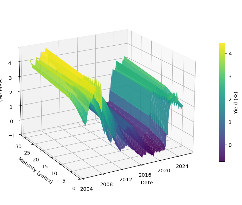
Figure 1, source Bloomberg

The Nelson Siegel Model

Diebold and Li (2006) have used a modified Nelson Siegel model to predict bond yields and found it to be a superior model for predicting one year ahead. Modelling the yield curve is a complex task, the Nelson Siegel model tries to approximate the model of the yield curve by using a three-factor exponential model.

\( Y_t^{(c)}(\tau) = \beta_{1,t}^{(c)} + \beta_{2,t}^{(c)} (\frac{1 - e^{-\lambda \tau}}{\lambda \tau}) + \beta_{3,t}^{(c)} (\frac{1 - e^{-\lambda \tau}}{\lambda \tau} - e^{-\lambda \tau}) + \varepsilon_t^{(c)}(\tau), \)

The parameter λ_t controls the exponential decay rate. Small values of this parameter imply a slow decay rate, while large values imply a fast decay rate. A small value of λ_t is better at modelling long term bond and a large value of λ_t fits better with a short term bond. Diebold and Li (2006) uses a value λ_t = 0.0609, their models view maturities in months. In my model we view maturities in years, so I use 12∗λ_t. The beta vectors β^(c)_t are estimated by (cross-sectional) ordinary least squares. This yields a time series of estimated vectors for each country:

\( \bigl\{\hat{{\beta}}^{(c)}_t\bigr\}_{t=1}^T. \)

A more detailed derivation for interested readers can be found in the Appendix A1. The yield curve is fitted at each data point available. For illustration, in Figure 2, four different dates in Germany’s yield curve history are presented with the fitted Nelson Siegel model.

Figure 2

Predictions

Now we use our fitted Nelson Siegel models to predict future bond yields. In particular, we predict the coefficients {βˆ_{1t}, βˆ_{2t}, βˆ_{3t}} using an AR(p) model. Diebold and Li (2006) use an AR(1) model to predict future bond yields. They found that predicting 12 months ahead gave the best results. For my prediction I use the Akaike Information Criterion (AIC) to select the amount of lags used in each model. The amount of lags p will differ per country and the AR(p) model is defined as:

\(\beta_{it} = c_i + \sum_{j=1}^{p}\phi_{ij}\beta_{i,t-j} + \varepsilon_{it}, \qquad i=1,2,3.\)

The h-step-ahead factor forecasts βˆ_{i,t+h|t} are then inserted into the Nelson Siegel formula to obtain the forecasted yield curve:

\(\hat{y}_{t+h\mid t}(\tau) = \hat{\beta}_{1,t+h\mid t} + \hat{\beta}_{2,t+h\mid t}\left(\frac{1-e^{-\lambda \tau}}{\lambda \tau}\right) + \hat{\beta}_{3,t+h\mid t}\left(\frac{1-e^{-\lambda \tau}}{\lambda \tau}-e^{-\lambda \tau}\right).\)

We apply the above to obtain our prediction, Figure 3 presents the resulting prediction for Germany’s yield curve.

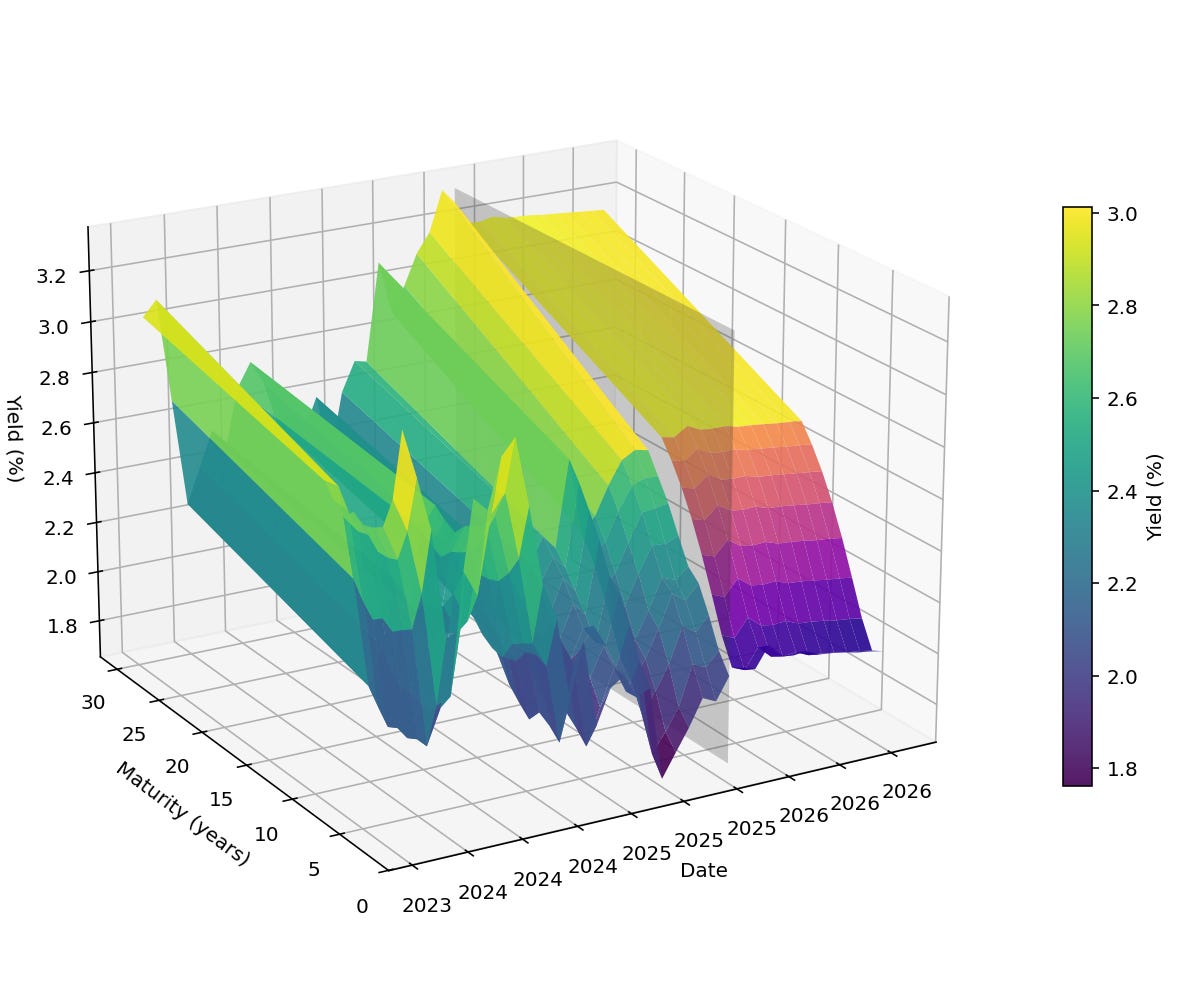
Figure 3

Investigating Spreads

The main interest for us is to inspect the spreads of countries in the EU. By forecasting the yield curve for Germany, Italy, and France, spreads can be constructed by subtracting these curves. In Figure 4 we see the forecasted spread of Italy-Germany 10YR. In Figure 5 the France-Germany 10YR maturity spread is forecasted. The model predicts a small decrease in the spread. Since the prediction is based on a AR(p) model it will not give big shocks as predictions.

In Figure 6 the German 10YR-2YR curve is forecasted. Once again the forecast is quite flat with a small predicted decrease.

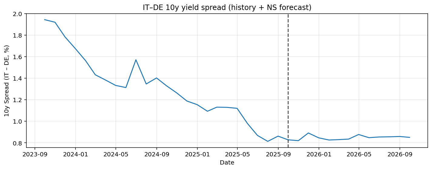
Figure 4

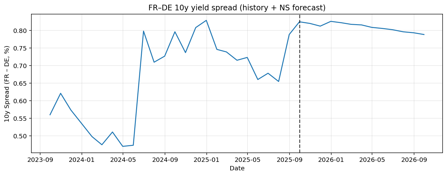
Figure 5

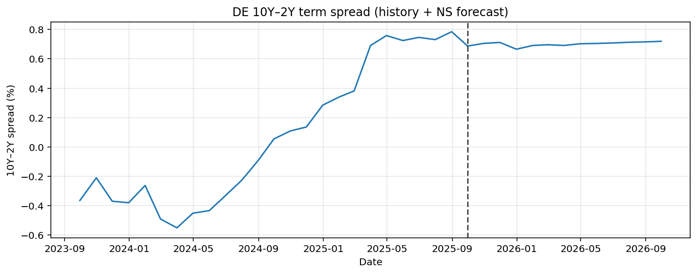
Figure 6

Prediction Uncertainty

We have some predictions, but are they any good?

When forecasting it is always a good practice to include uncertainty in the predictions. Therefore, I will include bootstrapped confidence intervals that do not make distributional assumptions. This will cause the confidence intervals to be wider compared to standard normally distributed intervals, but yield more realistic confidence intervals. The method used specifically is called a ‘Sieve’ bootstrap. A more detailed explanation is in the appendix A2.

The Italy-Germany and France-Germany 10YR spread including bootstrapped 95% confidence intervals are given in Figure 7 and Figure 8. For both spread predictions the point forecast only predicts limited variation in the future, while the confidence interval is relatively wide. This implies there is significant uncertainty in the prediction. The confidence intervals are also asymmetric. For the Italy-Germany case there is more possibility to the upside of the prediction. For the France-Germany case it is quite the opposite, the risks are more skewed to the downside.

Overall, the bootstrap results suggest that while no strong deterministic changes in spreads are predicted, the distribution of future outcomes is skewed, highlighting directional risks that are not apparent from point forecasts.

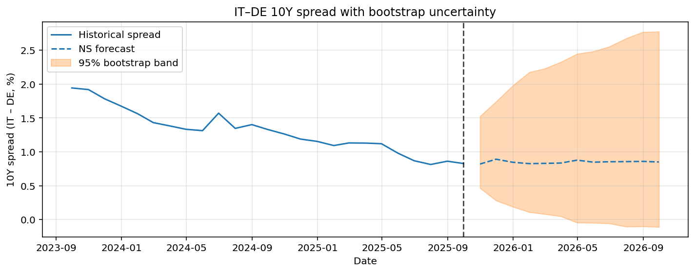
Figure 7

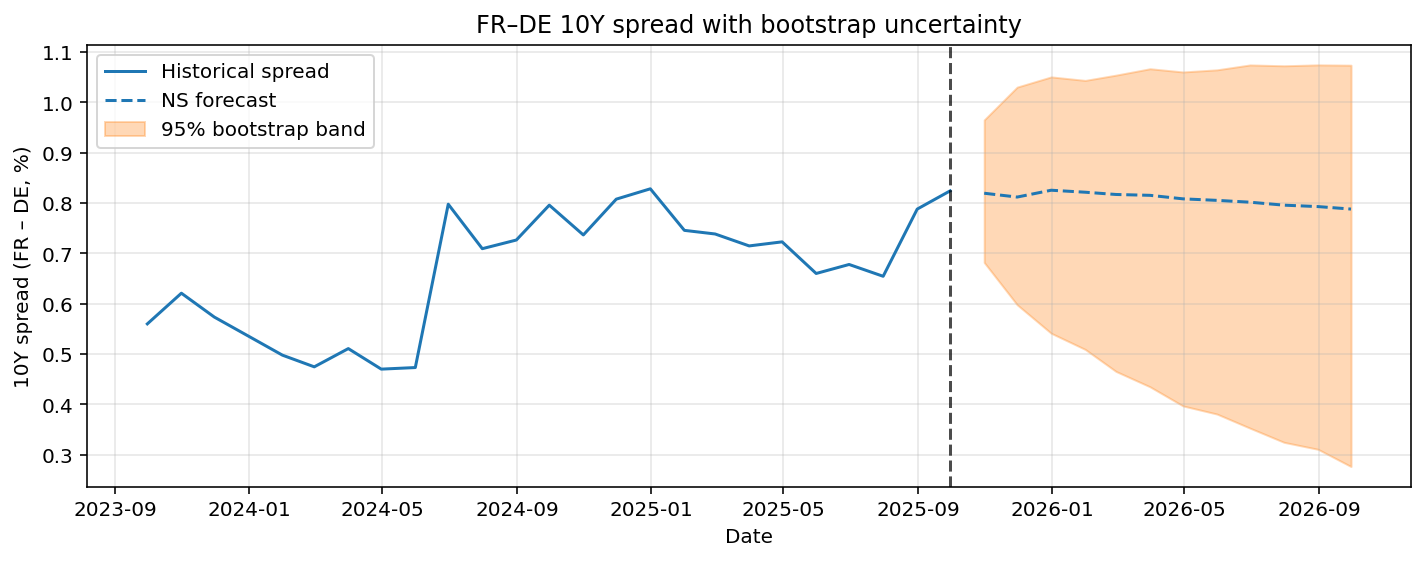
Figure 8

Findings

In this article, a Nelson Siegel model is used to forecast government bond yield curves and yield spreads for Germany, France, and Italy. The model fits the historical yield curves reasonably well, but the point forecasts themselves are mostly flat over the next year and come with a lot of uncertainty. The more interesting results come from the confidence bands. These bands are wide and clearly asymmetric, meaning that the risks are not evenly balanced. For some spreads, there is more risk on the upside, while for others the downside risk dominates. This shows that even when the expected change in spreads is small, the direction of risk can still matter. Overall, this type of model is better suited for understanding uncertainty and risk around yield spreads than for making precise point predictions.

Appendix

A1 Nelson Siegel Model

We consider zero-coupon yields observed at discrete times t = 1, …, T, for multiple countries and maturities.

Let

\( Y_t^{(c)}(\tau) \)

denote the yield at time t for country c and maturity τ > 0 (in years), e.g. τ_j ∈ {2, 3, 4, 5, 6, 7, 8, 9, 10, 30} years. For each country c and time t, we assume a Nelson Siegel representation of the yield curve.

\(Y_t^{(c)}(\tau) = \beta_{1,t}^{(c)} + \beta_{2,t}^{(c)} (\frac{1 - e^{-\lambda \tau}}{\lambda \tau}) + \beta_{3,t}^{(c)} (\frac{1 - e^{-\lambda \tau}}{\lambda \tau} - e^{-\lambda \tau}) + \varepsilon_t^{(c)}(\tau),\)

The parameter λ_t controls the exponential decay rate. Small values of this parameter imply a slow decay rate, while large values imply a fast decay rate. A small value of λ_t is better at modelling longer term bonds and a large value of λ_t fits better with a shorter term bonds. Diebold and Li (2006) uses a value λ_t = 0.0609, their model views maturities in months. In my model we view maturities in years, so I use 12 ∗ λ_t. Now all we have left are the betas. Using ordinary least squares the coefficients { βˆ_{1t}, βˆ_{2t}, βˆ_{3t} } are estimated for each point in time. At each observation we fit the Nelson Siegel model to fit the yield curve at that moment. For illustration, I show the fitted yield curve model at four specific data points in Figure 2. As you can see the fitted Nelson Siegel model fits reasonably well. It is also noteworthy that I do not posses the data of more short term maturity bonds. This creates a different yield curve image compared to yield curves that include maturities below two years. The model can be written as a vector model.

\(Y_t^{(c)}(\tau_j) \approx \beta_{1,t}^{(c)} f_1(\tau_j;\lambda) + \beta_{2,t}^{(c)} f_2(\tau_j;\lambda) + \beta_{3,t}^{(c)} f_3(\tau_j;\lambda), \quad j = 1,\dots,J.\)

Define the factor loading vector as

\({f}(\tau_j; \lambda) = \begin{pmatrix} f_1(\tau_j; \lambda)\\ f_2(\tau_j; \lambda)\\ f_3(\tau_j; \lambda) \end{pmatrix} \in \mathbb{R}^3,\)

and the time-t Nelson Siegel beta vector

\({\beta}_t^{(c)} = \begin{pmatrix} \beta_{1,t}^{(c)}\\ \beta_{2,t}^{(c)}\\ \beta_{3,t}^{(c)} \end{pmatrix} \in \mathbb{R}^3.\)

Then for a given t and c, the model can be written compactly as

\({y}_t^{(c)} = F(\lambda)\, {\beta}_t^{(c)} + {\varepsilon}_t^{(c)},\)

where

\({y}_t^{(c)} = \begin{pmatrix} Y_t^{(c)}(\tau_1)\\ \vdots\\ Y_t^{(c)}(\tau_J) \end{pmatrix}, \quad F(\lambda) = \begin{pmatrix} {f}(\tau_1;\lambda)^\top\\ \vdots\\ {f}(\tau_J;\lambda)^\top \end{pmatrix} \in \mathbb{R}^{J \times 3}.\)

as mentioned before, given the observed yields y^{(c)}_t and fixed λ, the Nelson Siegel betas β^{(c)}_t are estimated by (cross-sectional) ordinary least squares. This yields a time series of estimated Nelson Siegel factor vectors for each country:

\(\bigl\{\hat{{\beta}}^{(c)}_t\bigr\}_{t=1}^T.\)

A2 Confidence intervals

We will perform a ’Sieve’ bootstrap that takes parameter uncertainty of the AR(p) model into account, as well as the prediction uncertainty. The main idea is to redraw the errors of the fitted AR(p) process with replacement. Using the errors new AR(p) models are estimated and with the bootstrapped models we obtain new predictions. The 95% confidence interval of the bootstrapped predictions will give us a quantified measure of the parameter and prediction uncertainty. Now we will use some mathematical definitions for the bootstrap method.

The stacked beta vector b_t ∈ R^6 (Two countries stacked) is modelled as

\(b_t = \mu + \sum_{i=1}^p A_i b_{t-i} + e_t,\)

with residuals eˆ_t from the estimated model.

Let

\(\tilde e_t = \hat e_t - \bar e, \qquad \bar e = \frac{1}{T-p} \sum_{s=p+1}^T \hat e_s,\)

and let

\(\{\tilde e_t\}_{t=p+1}^T\)

be the empirical residual pool.

For each bootstrap replication b = 1, . . . , B we:

1. Generate a pseudo sample

   \(\{b_t^{*(b)}\}_{t=1}^T\)

   recursively by

   \(b_t^{*(b)} = \hat\mu + \sum_{i=1}^p \hat A_i\, b_{t-i}^{*(b)} + e_t^{*(b)}, \qquad e_t^{*(b)} \in \{\tilde e_{p+1},\dots,\tilde e_T\}\)

   where the residuals e^{∗(b)}_t are drawn with replacement from the residual pool, and the first p values b^{∗(b)}_1 , …, b^{∗(b)}_p are set equal to the observed b_1, …, b_p.

2. Re-estimate the VAR(p) on {b^{∗(b)}_t} to obtain bootstrap parameters μˆ^{∗(b)} and Aˆ^{∗(b)i} .

3. Starting from b^{∗(b)}_T, simulate a bootstrap forecast path b^{∗(b)}_{T+1}, …, b^{∗(b)}_{T+h} using

   \(b_{T+k}^{*(b)} = \hat\mu^{*(b)} + \sum_{i=1}^p \hat A_i^{*(b)}\, b_{T+k-i}^{*(b)} + \eta_{T+k}^{*(b)},\)

where each η^{∗(b)}_{T+k} is again drawn with replacement from the centred residuals {˜e_t}. For each b and k, the corresponding Nelson Siegel beta vectors are mapped back to yields via the Nelson Siegel formula and then to term spreads and cross-country spreads. The empirical quantiles of the bootstrap forecasts

\(\{S_{T+k}^{*(b)}\}_{b=1}^B,\quad \text{or} \quad \{T_{T+k}^{*(b)}\}_{b=1}^B\)

provide bootstrap prediction intervals, for example the 2.5% and 97.5% quantiles yield a 95% prediction band.

References

Diebold, Francis X. and Canlin Li (2006). Forecasting the term structure of government bond yields. Journal of Econometrics 130 (2), 337–364.